Introduction
A few years ago I came across this paper by Michael W. Dorrity and Lauren M. Saunders et. al. who used dimensionality reduction (DR) techniques to infer protein complexes and pathways from a dataset of 1,484 single gene deletions in the yeast genome. They used a DR algorithm called Uniform Manifold Approximation and Projection (UMAP) and showed that UMAP distance identifies protein interactions more effectively than other methods, including pairwise correlation. Genetic knockout experiments are a great way to assess gene function, with experimental techniques such as Pertub-seq allowing us to analyse transcriptional profiles of gene perturbations at scale. This however remains very expensive, and publications often perturb just a handful of genes, which is why I was really excited when I came across an algorithm called scTenifoldKnk, developed by Daniel Osorio et al, which allows you to perform virtual knockout (KO) experiments using scRNAseq data.
Understanding scTenifoldKnk
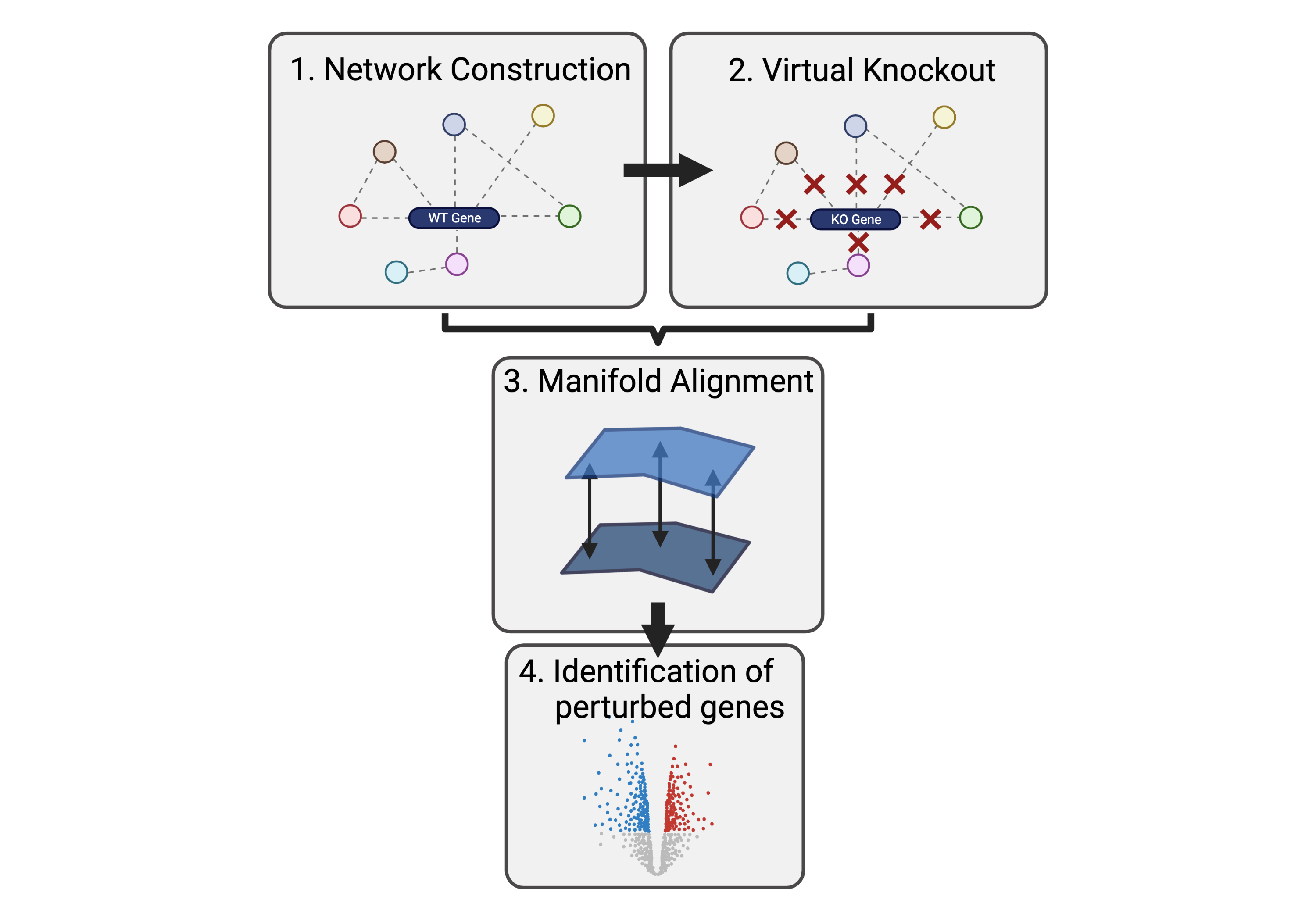
scTenifoldKnk uses wild-type (WT) scRNAseq data to construct a gene regulatory network (GRN) consisting of genes (nodes) and their connections (edges). Any particular gene can then be virtually knocked out by converting its outward edge weights to zero (Figure 1). Differential regulation of genes can then be inferred from the comparison between the WT and KO GRNs. But here comes the cool bit, instead of directly analysing changes in the edge weights of the GRNs, the algorithm employs quasi-manifold alignment to learn hidden representations of the two networks, aligning them, and comparing the distance between a gene in the low dimensional representation of the networks. The greater the distance between a gene in the WT and KO manifold the more significant is its differential regulation. Similar to the paper mentioned above, the authors show that the manifold representation of the GRNs is an essential step to find biologically meaningful gene interactions. Moreover, they validate scTenifoldKnk using various comparisons to real world KO experiments and mendelian diseases. My explanation of the algorithm is quite simplified so if you would like to understand more about the algorithm, I would highly recommend you read this paper describing it.
Virtual KO of all expressed genes in CD4 T cells
As described in their paper, we can use scTenifoldKnk to systematically perturb all genes in a scRNAseq dataset and then use the distance metric to perform dimensionality reduction on all perturbations to hopefully infer protein interactions from its clustering.
Data Preprocessing
Before we can send our script off to individually knockout all the genes (the fun bit), we need to download and clean our data (the necessary bit). In this paper Eddie Cano-Gamez et. al. sequenced 40,000 naive and memory CD4 T cells to elucidate an effectorness gradient which shapes their response to cytokines, the data of which can be downloaded from here. They used the 10x Genomics 3’ v2 chemistry to sequence CD4 T cells which were stimulated with various cytokines to polarise them towards various helper T cell phenotypes. They then used the cellranger pipeline to align reads to the hg38 build of the human genome.
So we can start off by loading the Seurat library which we will use to preprocess the data, setting our random seed and setting our working directory.
# Load packages
library(Seurat)
library(magrittr)
library(tidyverse)

set.seed(1234)

setwd('./VirtualKO_Gamez_CD4/')
We can now create a seurat cell data set using our downloaded sequencing and metadata.
# Read raw data and metadata
raw_data <- Read10X(data.dir ='./GRCh38/', gene.column = 1)
metadata <- read.table('./NCOMMS-19-7936188_metadata.txt', fill = T, row.names = 1, sep = '\t')

# Create new cell data set
cds <- CreateSeuratObject(raw_data, min.cells = 3,
                          project = 'Gamez_CD4',
                          assay = 'RNA',
                          meta.data = metadata)

# Remove raw_data object to save space
rm(raw_data)
We can now assign further metadata variables to our cell data set and filter out the cytokine conditions and celltypes we are interested in. For now we’ll only look at Naive (N), Central Memory (CM), Effector Memory (EM) and Effector Memory re-expressing CD45RA (EMRA) cells in either unstimulated or stimulated with anti-CD3/CD28 bead conditions. We can then filter out cells that contain more than 8000 features and those that have more than 20% of reads mapped to mitochondrial genes.
# Create new celltype metadata variable
cds[['celltype']] <- sub('(.*)[1,2]', '\\1', sub('(.*) .*','\\1',cds@meta.data$cluster.id))

# Filter unstimulated and stimulated cells, as well as N/CM/EM/EMRA cells
cds <- subset(cds, subset = (cytokine.condition == 'UNS' | cytokine.condition == 'Th0') & celltype %in% c('TN', 'TCM', 'TEM', 'TEMRA'))

# Create new stim metadata variable
cds[['stim']] <- ifelse(cds@meta.data$cytokine.condition == 'UNS', 'CTRL', 'STIM')

# Calculate mitochondrial content per cell
cds[["percent.mt"]] <- PercentageFeatureSet(cds, pattern = "^MT-")

# Filter cells by features and mitochondrial content
cds <- cds %>%
  subset(subset = nFeature_RNA < 8000 & percent.mt < 20)
To aid in our downstream analysis we will now integrate the unstimulated and stimulated datasets. If you want to learn more about scRNAseq data integration you can check out this seurat vignette.
# Split the cell data set by stimulation status
cds_list <- SplitObject(cds, split.by = 'stim')

# Transform each group of cells individually
cds_list <- lapply(X = cds_list, FUN = function(x) {
  x <- SCTransform(x, verbose = FALSE)
})

# Perform integratiion
features <- SelectIntegrationFeatures(object.list = cds_list, nfeatures = 3000)
cds_list <- PrepSCTIntegration(object.list = cds_list, anchor.features = features)
reference_dataset <- which(names(cds_list) == 'CTRL')
anchors <- FindIntegrationAnchors(object.list = cds_list, normalization.method = 'SCT',
                                  anchor.features = features, k.anchor = 20, reference = reference_dataset)
cds_int <- IntegrateData(anchorset = anchors, normalization.method = 'SCT')

# Set the integrated dataset as the default assay
DefaultAssay(cds_int) <- "integrated"
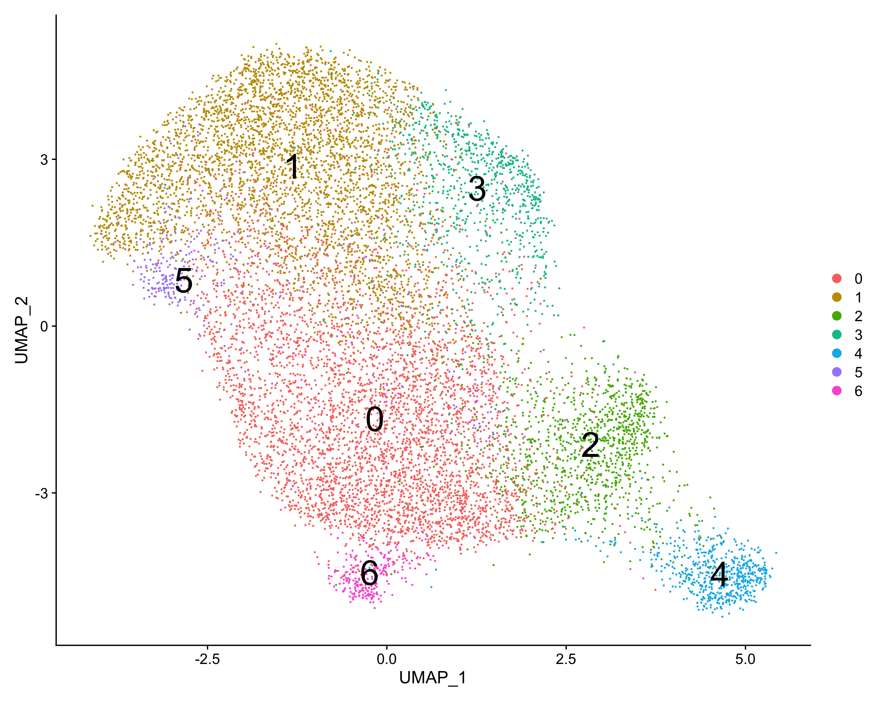
Now that our data is integrated, we can scale our data, apply dimensionality reduction and cluster the cells. Because we will not make much use of this clustering and dimensionality reduction in our downstream analysis I will not go into selecting the optimal number of dimensions.
# Perform data scaling, dimensionality reduction and clustering
cds_int <- cds_int %>%
  ScaleData(verbose = FALSE) %>%
  RunPCA(npcs = 30, verbose = FALSE) %>%
  RunUMAP(reduction = "pca", dims = 1:30) %>%
  FindNeighbors(reduction = "pca", dims = 1:30) %>%
  FindClusters(resolution = 0.5)

# Plot UMAP
DimPlot(cds)
We have now finished preprocessing our data and can export the non-integrated count data and save the R session. Here we also filter out mitochondrial and ribosomal genes, after which we are left with expression data of 11,337 genes across 20,487 cells.
# Extract RNA counts
tmp <- as.matrix(cds@assays$RNA@counts)

# Filter mitochondrial and ribosomal genes
tmp <- tmp[!grepl('^MT-|^RPL|^RPS',rownames(tmp), ignore.case = TRUE),]

# Show final matrix dimensions
dim(tmp)

# Export the count matrix and save the R session
write.table(tmp, './Gamez_CD4_scRNAseq_count_matrix.txt')
save.image(file='Gamez_CD4_T_cells.RData')
Systematic KO using scTenifoldKnk
scTenifoldKnk can be run locally on your computer, however to save time I will send the below sript to our university high performance compute cluster. The script is a modified version of the scTenifoldKnk package on github which relies on scTenifoldNet. It generates the gene regulatory network, and conducts manifold alignment and differential regulation analysis in a parallelised manner. The function for differential regulation analysis (dRegulation) will need to be saved in your directory in order for the script to be able to load it. The script also scales the distances between genes from the manifold alignmennt for each gene KO in our data.
################################################################################
## Systematic KO of CD4 T cell Transcriptome
################################################################################


# Setup ------------------------------------------------------------------------

# Set working directory
setwd('./')

# Set random seed
set.seed(1234)

# Load required packages
library(foreach)
library(doSNOW)
library(magrittr)

# Load dRegulation function
source('./dRegulation.R')

print('Setup Complete')

# Data Loading & Preprocessing -------------------------------------------------

# Load data
countMatrix <- read.table('./Gamez_CD4_scRNAseq_count_matrix.txt')

# Filter genes with a mean gene count of >= 0.05
countMatrix <- countMatrix[rowMeans(countMatrix != 0) >= 0.05,]

print('Preprocessing Complete')

# Gene Regulatory Network ------------------------------------------------------

# Construct gene regulatory network
WT <- scTenifoldNet::makeNetworks(X = countMatrix,
                                  q = 0.9,
                                  nNet = 10,
                                  nCells = 500,
                                  scaleScores = T,
                                  symmetric = F,
                                  nComp = 3,
                                  nCores = as.integer(Sys.getenv('NSLOTS')))
# Tensor decoposition
WT <- scTenifoldNet::tensorDecomposition(xList = WT,
                                         K = 3,
                                         maxError = 1e-05,
                                         maxIter = 1000,
                                         nDecimal = 3)
# Preprocessing
WT <- WT$X
S <- as.matrix(WT)
S[abs(S) < abs(t(S))] <- 0
O <- (((1-0) * WT) + (0 * S))
WT <- as.matrix(O)
diag(WT) <- 0
WT <- t(WT)

save.image(file='./Results/GenomeWideKO.RData')

print('WT GRN Complete')

# Setup Parallel ---------------------------------------------------------------

# Register cluster for parallelisation
my.cluster <- parallel::makeCluster(as.integer(Sys.getenv('NSLOTS')))
doParallel::registerDoParallel(cl = my.cluster)

print(paste('Parallel Cores Registered =', foreach::getDoParRegistered(),'-', foreach::getDoParWorkers(), 'Cores Detected'))

# Progress Bar -----------------------------------------------------------------

# Generate progress bar to track progress
registerDoSNOW(my.cluster)
pb <- txtProgressBar(max = nrow(WT), style = 3)
progress <- function(n) setTxtProgressBar(pb, n)
opts <- list(progress = progress)


# Genome Wide Differential Regulation ------------------------------------------

# New matrix to store results
gw_DR <- matrix(ncol = 7, dimnames = list(NA, c('gKO', 'gene', 'distance', 'Z', 'FC', 'p.value', 'p.adj')))

start_time_to <- Sys.time()

# Parallelised for loop to obtain differential regulation comparing WT to each KO gene
gw_DR <- foreach(i = rownames(WT),
                 .combine = rbind,
                 .packages = c('scTenifoldNet'),
                 .options.snow = opts
) %dopar% {

  # Copy WT GRN to KO GRN
  KO <- WT

  # Zero out edge weights of knockout gene
  KO[i,] <- 0

  # Align WT and KO manifolds
  MA <- scTenifoldNet::manifoldAlignment(X = WT,
                                         Y = KO,
                                         d = 2,
                                         nCores = 1)

  # Perform differential regulation analysis
  DR <- dRegulation(MA, i)

  return(cbind('gKO' = i, DR))

}

save.image(file='./Results/GenomeWideKO.RData')

paste('Differential regulation calculated in:', round(difftime(Sys.time(), start_time_to, units = 'm'), 0), 'min')


# Scaling of Genome Wide Knockout Distances ------------------------------------

# New matrix to store knockout-wise gene distances
gw_KO <- matrix(nrow = nrow(WT),
                ncol = ncol(WT),
                dimnames = list(rownames(WT)))

start_time <- Sys.time()

# Parallelised for loop to scale gene distancces
gw_KO <- foreach(i = rownames(WT),
                 .combine = cbind,
                 .packages = c('MASS', 'magrittr', 'dplyr'),
                 .options.snow = opts
) %dopar% {

  # Filter gene of interest
  tmp <- gw_DR %>%
    dplyr::filter(gKO == i)

  # Make 'tmp' available in the global environment
  .GlobalEnv$tmp <- tmp

  # Calculate optimal lambda
  b <- MASS::boxcox(lm(tmp$distance ~ 1), plotit = F)
  lambda <- b$x[which.max(b$y)]

  # Boxcox transform distance
  tmp <- tmp %>%
    dplyr::mutate(dist_scaled = scale(EnvStats::boxcoxTransform(distance, lambda = lambda)))

  return(tmp[match(rownames(gw_KO), tmp$gene),'dist_scaled'])
}

# Assign row and column names
rownames(gw_KO) <- rownames(WT)
colnames(gw_KO) <- paste0(rownames(WT), '_gKO')

save.image(file='./Results/GenomeWideKO.RData')

paste('KO distances scaled in:', round(difftime(Sys.time(), start_time, units = 'm'), 0), 'min')

parallel::stopCluster(my.cluster)

# Export files -----------------------------------------------------------------

write.table(as.data.frame(gw_DR), './Results/GenomeWide_DR.txt', col.names = T, row.names = F)
write.table(as.data.frame(gw_KO), './Results/GenomeWide_KO.txt', col.names = T, row.names = T)

save.image(file='./Results/GenomeWideKO.RData')
Depending on whether you have access to a high performance compute cluster this can be a great way to save you from leaving your laptop running for days on end. The above script can then be submitted to the cluster via the below shell script.
#!/bin/bash
#$ -wd ./VirtualKO/
#$ -j y
#$ -pe smp 12
#$ -l h_rt=24:0:0
#$ -l h_vmem=8G
#$ -N genome_wide_ko
#$ -m beas

module load R

Rscript GenomeWideKO.R