Environment Setup
library(Seurat)
library(magrittr)
library(dplyr)
Data Import and Preprocessing
Read data generated by cellranger count/aggregate. Create seurat object, filtering out all genes expressed in less than 3 cells and all cells with less than 200 expressed genes
raw_data <- Read10X(data.dir = '.../filtered_gene_bc_matrices/hg19/')

cds <- CreateSeuratObject(raw_data,
                          min.cells = 3,
                          min.features  = 200,
                          project = "10X_CD8",
                          assay = "RNA")

rm(raw_data)
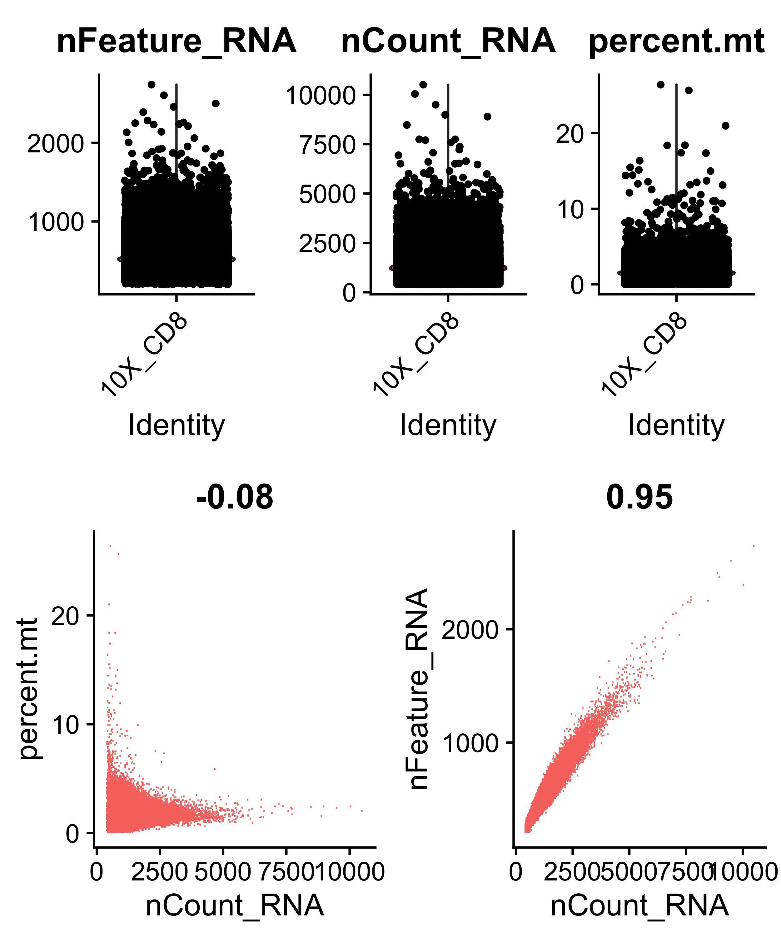
Calculate percent mitochondrial gene expression per cell, plot diagnostic plots, and filter cells with than 400 and less than 1500 genes, and cells with less than 5% mitochondrial gene expression (cells with more than 5% are low quality).
cds[["percent.mt"]] <- PercentageFeatureSet(cds, pattern = "^MT-")

VlnPlot(object = cds, features = c("nFeature_RNA", "nCount_RNA", "percent.mt"), ncol = 3)
FeatureScatter(object = cds, feature1 = "nCount_RNA", feature2 = "percent.mt")
FeatureScatter(object = cds, feature1 = "nCount_RNA", feature2 = "nFeature_RNA")

cds <- subset(x = cds, subset = nFeature_RNA > 400 & nFeature_RNA < 1500 & percent.mt < 5 )
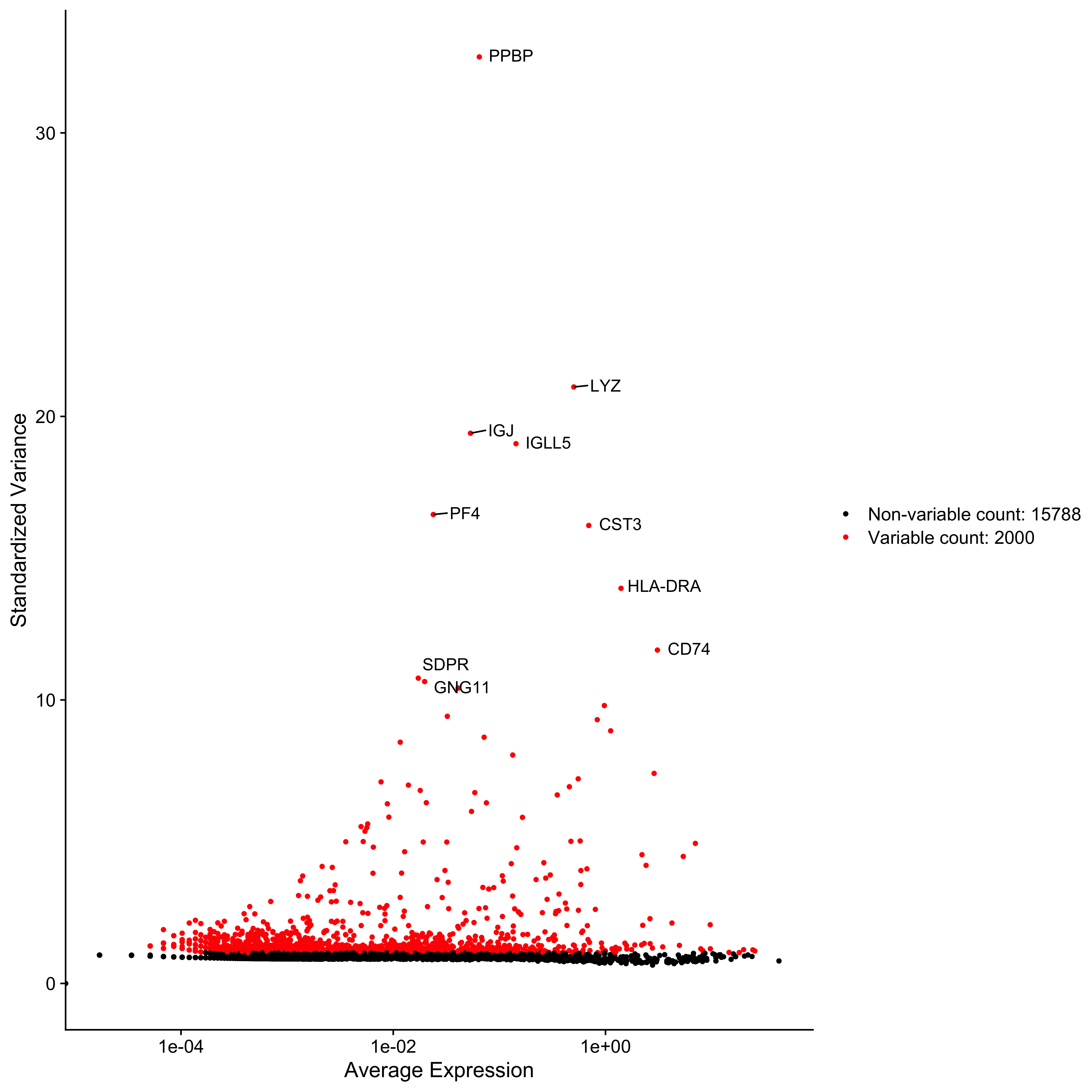
Normalise and scale the data. Followed by calculating all variably expressed genes and selecting the top ten differentially expressed ones and plotting them.
cds <- NormalizeData(cds)
cds <- ScaleData(cds, features = rownames(cds))

cds <- FindVariableFeatures(cds, selection.method = "vst", nfeatures = 2000)

top10 <- head(VariableFeatures(cds), 10)

plot1 <- VariableFeaturePlot(cds)
LabelPoints(plot1, top10, repel = TRUE)
Dimensionality Reduction and Clustering
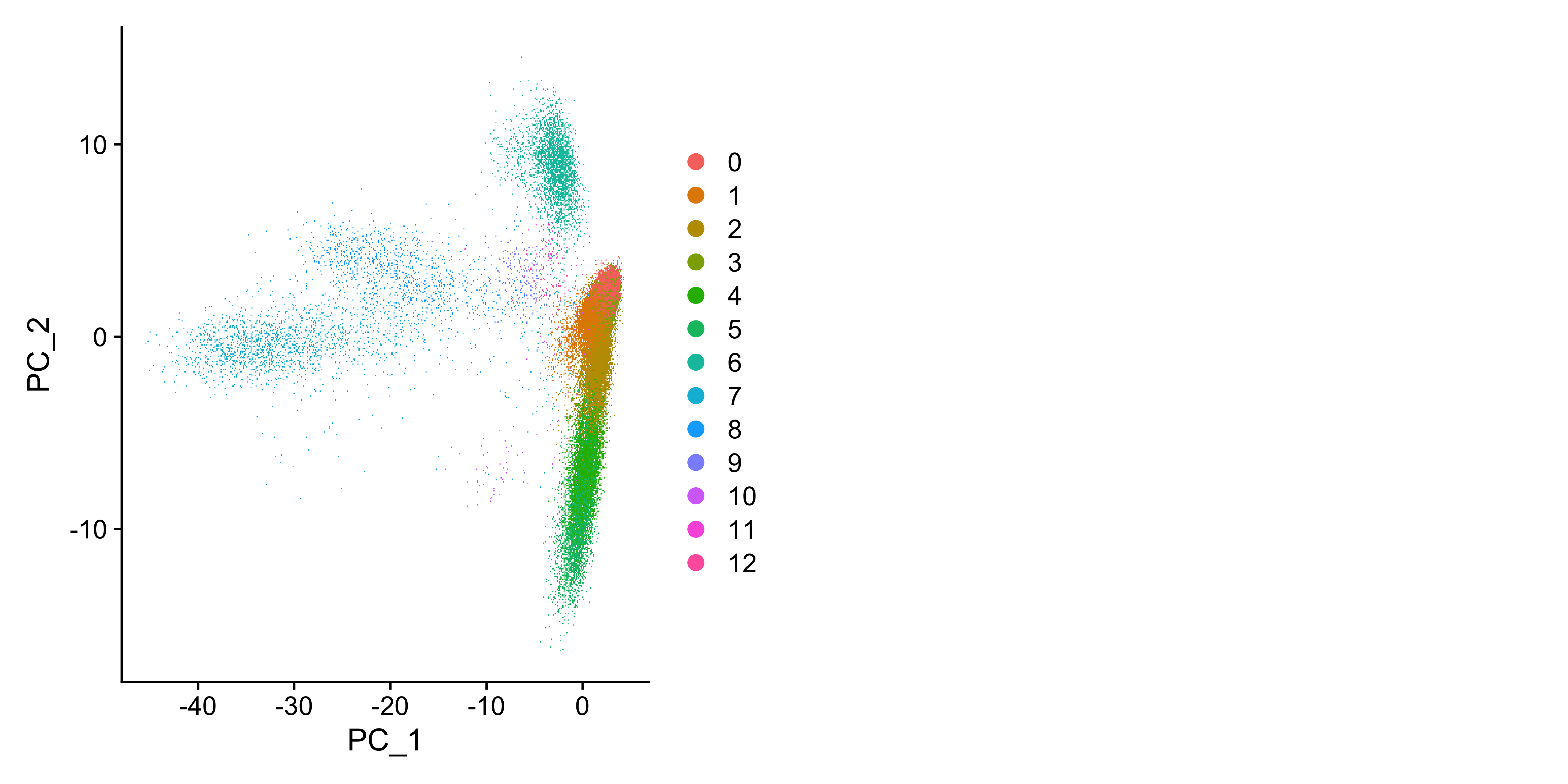
First we run a PCA for an initial dimensionality reduction, which we will later load into UMAP.
cds <- RunPCA(cds)

print(cds[["pca"]], dims = 1:5, nfeatures = 5)
VizDimLoadings(cds, dims = 1:2, reduction = "pca")

DimPlot(object = cds, reduction = "pca")
DimHeatmap(object = cds, reduction = "pca", cells = 200, balanced = TRUE)
# Find cluster number
ElbowPlot(object = cds)

# Clustering
cds <- FindNeighbors(cds, reduction = 'pca', dims = 1:15)
cds <- FindClusters(cds, resolution = 0.5, algorithm = 1)

# UMAP dim reduction
cds <- RunUMAP(cds, reduction = "pca", dims = 1:15)

DimPlot(cds, reduction = "umap")

# Find all variable markers between clusters
markers <- FindAllMarkers(cds)

# Top 5 Clusters per marker
top5 <- markers %>% group_by(cluster) %>% top_n(5, avg_logFC)

# Plotting
DoHeatmap(object = cds, features = top5$gene, label = TRUE)

FeaturePlot(object = cds, features = top5$gene, cols = c("grey", "red"), reduction = "umap")

# Specific gene ex. CD27
DoHeatmap(object = cds, features = 'CD27', label = TRUE)


## Monocle for Trajectory inference ----
## https://cole-trapnell-lab.github.io/monocle3/docs/starting/

library(monocle3)

path <- '.../RNAseq analysis/CD8 T cells'

cds <- load_cellranger_data(path)

cds <- preprocess_cds(cds)
plot_pc_variance_explained(cds)

cds <- align_cds(cds)

cds <- reduce_dimension(cds)

cds <- cluster_cells(cds)
plot_cells(cds, color_cells_by = 'cluster')

cds <- learn_graph(cds)
cds <- order_cells(cds)

plot_cells(cds, color_cells_by="pseudotime", label_cell_groups=FALSE)